Building the motor model
Two coupled equations, one parameter set and an independent steady-state check.
Before you begin: matrix equations, Laplace transforms and complex roots.
After this lesson you can: derive transfer functions, find system time scales and justify a reduced model.
Work through the explanation, examples, practical experiment and independent exercises.
- Object and assumptions
- Coupled equations
- Find equilibrium first
- Isolated and coupled time scales
- The right-hand side
- State space and the exact interval solution
- Voltage and load transfer functions
- Poles and damping
- When inductance can be neglected
- Independent exercises
- Practical work
- Calculated illustrations
- Key takeaways
Object and assumptions
Our teaching object is a constant-flux DC motor with a rigid shaft. Parameters illustrate dynamics rather than represent a particular product. We omit temperature rise, saturation, brush drop, PWM ripple, dry friction and shaft flexibility. A real machine needs measured or documented parameters and experimental model validation.
b = 0.002 N·m·s/rad; kt = 0.1 N·m/A; ke = 0.1 V·s/rad
Base input U = 12 V
Coupled equations
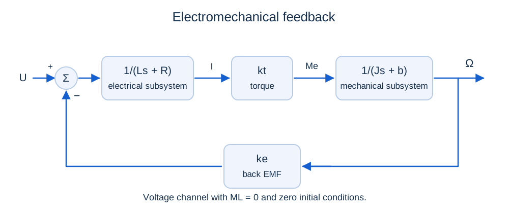
ω′ = (kti − bω − ML)/J
Startup from rest uses i(0) = 0 A and ω(0) = 0 rad/s. When continuing across a switch, transfer both final states from the previous interval. Do not reset the motor at each event.
Find equilibrium first
i∞ = (bω∞ + ML)/kt
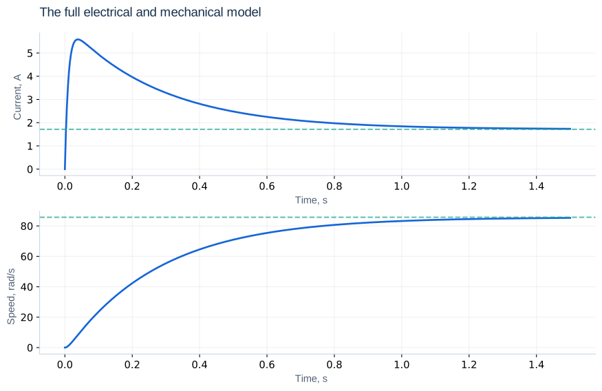
With no external load, ω∞ = 85.714 rad/s and i∞ = 1.714 A. Current is nonzero because it supplies viscous friction. At ML = 0.1 N·m, speed falls to 71.429 rad/s and current rises to 2.429 A. Starting current rises quickly and later falls as back EMF develops. Monotonic speed in this example is not a universal property of every parameter set.
Isolated and coupled time scales
L/R = 0.01 s and J/b = 1 s describe isolated electrical and mechanical subsystems. The coupled motor has poles near −97.407 and −3.593 s⁻¹, corresponding to 0.0103 and 0.278 s. Internal electromechanical feedback changes the decay rate; J/b alone is not a motor starting-time estimate.
The right-hand side
def motor(t, y, voltage=12.0, load=0.0):
    i, w = y
    R, L, J, b, k = 2.0, 0.02, 0.002, 0.002, 0.1
    return [(voltage-R*i-k*w)/L,
            (k*i-b*w-load)/J]
For piecewise-constant inputs, integrate separate intervals and carry the state forward. This makes switching times explicit.
State space and the exact interval solution
A = [−R/L, −ke/L; kt/J, −b/J]
B = [1/L, 0]ᵀ; E = [0, −1/J]ᵀ
x∞ = −A⁻¹(BU + EML)
x(t) = x∞ + exp(At)(x₀ − x∞)
The semicolon separates matrix rows. For constant parameters the system is linear and time invariant. When A is invertible and inputs constant, the matrix exponential provides an independent numerical reference.
Voltage and load transfer functions
Ω(s) = [kt/D(s)]U(s) − [(Ls + R)/D(s)]ML(s)
I(s) = [(Js + b)/D(s)]U(s) + [ke/D(s)]ML(s)
These expressions assume zero initial conditions. Setting s = 0 recovers equilibrium. The load channel is negative for speed and positive for current. Outputs share poles but have different numerators, explaining their different response shapes.
Further reading: University of Michigan CTMS: DC motor model. Notation may differ from this course.
Poles and damping
ωn = √[(Rb + ktke)/(LJ)]
ζ = (R/L + b/J)/(2ωn)
The base polynomial is s² + 101s + 350. Its poles are −97.407 and −3.593 s⁻¹; ωn = 18.708 rad/s and ζ ≈ 2.699. The slow pole dominates duration, but modal amplitudes also depend on input, output and initial state.
When inductance can be neglected
Jω′ + (b + ktke/R)ω = (kt/R)u − ML
τeffective = J/(b + ktke/R) = 0.2857 s
This is useful after a fast electrical transient when mechanical motion and inputs are much slower. The full slow time is 0.2783 s, close to the approximation. However, the reduced model jumps to U/R at startup and loses current continuity. Validate it separately for current peaks, switching and fast current control.
Independent exercises
1. Find A, its trace and determinant for the base motor.
Show solution
A = [−100, −5; 50, −1]. Trace = −101 s⁻¹ and determinant = 350 s⁻². They equal the sum and product of eigenvalues.
2. Double J and estimate the new slow time.
Show solution
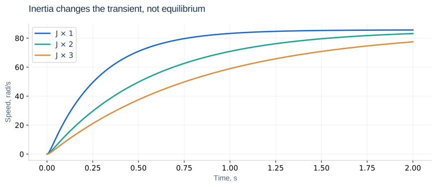
The polynomial is s² + 100.5s + 175. Poles are approximately −98.727 and −1.773 s⁻¹, giving 0.564 s. The reduced model gives 0.571 s.
Practical work
Simulate startup over 0–1.5 s and compare the endpoint with equilibrium. Triple J and extend the observation time: equilibrium stays unchanged. Compare full and reduced current and speed over 0–0.05 s and 0–2 s. A solver can accurately solve wrong equations, so use analytical checks.
Calculated illustrations
Key takeaways
Establish assumptions, parameters and equilibrium before computing a transient. Observe for long enough to capture the slowest mode.
Progress is stored only in this browser.